flowchart TB
  CL["Claim: the policy improved<br/>consumer welfare"] --> E1["Evidence A:<br/>model-based welfare bound"]
  CL --> E2["Evidence B:<br/>downstream real outcomes"]
  E1 --> F1["Fails if: preference class wrong,<br/>elicited p biased, worst case<br/>misdefined, shares mismeasured"]
  E2 --> F2["Fails if: control group invalid,<br/>outcome confounded, cohort<br/>composition changed"]
  F1 --> J{"Do the failure sets<br/>overlap?"}
  F2 --> J
  J -->|"Largely disjoint"| G["Agreement is informative:<br/>both would have to fail<br/>for different reasons"]
  J -->|"Shared assumption"| B["Agreement is nearly<br/>uninformative: one failure<br/>produces both results"]
73 Complementary Evidence and Triangulation
A welfare bound is an argument, and arguments can be wrong in ways that no amount of internal rigor detects. The bound of Chapter 72 rests on a model the authors wrote, a preference class they assumed, and survey moments they elicited. Each link is defensible; none is verifiable from inside the chain. What makes the conclusion believable is a second piece of evidence, produced by a different method, whose failure modes have nothing to do with the first.
This is what the anchor paper does in its final move. Having concluded from a calibrated model that restricting campus credit-card marketing raised student welfare, it goes back to the administrative records and asks a blunter question: did the students whose borrowing shifted actually do better in school? Final grade point averages rose about 2 percent and on-time graduation rates by nearly 10 percent among students from lower-income communities, relative to the top-income group whose borrowing was unaffected (Brown, Grodzicki, and Medina 2026). That result is looser and more suggestive than the model-based bound. It is also completely independent of it: no utility function, no elicited probability, no assumption about the preference class. If the model were wrong in some way the authors did not anticipate, there is no obvious reason grades would move.
This chapter is about designing that second leg deliberately rather than adding it opportunistically. It develops what makes evidence genuinely complementary, how the anchor study built three legs that fail for different reasons, why the third leg required a new identification strategy, and the inferential hazards— multiple outcomes, forking paths, correlated biases—that turn triangulation into an illusion of confirmation.
73.1 What Makes Evidence Complementary
Adding more evidence is not the same as adding independent evidence. A second specification of the same regression on the same data confirms that the first was computed correctly; it does not confirm that the design was valid. The useful criterion is about failure modes:
Two pieces of evidence are complementary for a claim when the assumptions that would have to fail for the first to be wrong are largely disjoint from the assumptions that would have to fail for the second.
Under that definition, robustness checks are usually not complementary, because they share the identifying assumption. A different outcome measured on the same design is partly complementary: it shares the design but not the measurement. A different design on a different data source measuring a different construct is fully complementary. Figure 73.1 makes the logic explicit.
There is a second, softer criterion that matters in practice: complementary evidence should be closer to the welfare object than the primary evidence, or else further from it but more directly observed. The model-based bound is close to welfare but heavily assumed; graduation rates are further from the concept of welfare but directly measured. Neither dominates, and the pairing is stronger than either.
73.2 The Three-Legged Design
The anchor study is best understood as three studies sharing a research question. Table 73.1 sets them side by side.
| Leg 1: administrative panel | Leg 2: matched survey | Leg 3: academic outcomes | |
|---|---|---|---|
| Question | Did the untargeted market move? | Why did it move, and were choices optimal? | Did the shift show up in real outcomes? |
| Data | Student-semester borrowing records | Survey linked to individual records | Student-level GPA, graduation, major |
| Design | Event-study DiD, freshmen as control | Cross-sectional regressions with record-based covariates | Cohort DiD, top-income quartile as control |
| Identifying assumption | Parallel trends between entering and continuing classes | Survey responses measure beliefs and knowledge validly | Cohorts before and after the rule comparable within quartile |
| Main threat | Recession confound differentially by class | Survey run years after the policy | Compositional change in who enrolls |
| What it cannot do | Say whether the shift helped | Establish causality | Isolate the mechanism |
The design lesson is in the last two rows. Every leg has a fatal-sounding weakness, and in each case the weakness is answered by a different leg rather than by a better version of the same leg. The survey cannot establish causality—so causality comes from the panel. The panel cannot establish welfare—so welfare comes from the model calibrated on the survey, and is corroborated by academic outcomes. The academic outcomes cannot identify a mechanism—so the mechanism comes from the survey.
73.2.1 Leg 2: linking survey responses to administrative records
The single most productive design choice in the study is unglamorous: the survey was administered to students at the same institution and matched to their administrative records. This converts a set of stated beliefs into a set of belief-versus-reality comparisons, which is a categorically different kind of measurement.
The payoff is visible in the departure that could not be detected any other way. Roughly a fifth of card-holding students who had taken student loans were unaware that additional loan capacity remained available to them, and students in that position were markedly more likely to borrow on their card (Brown, Grodzicki, and Medina 2026). Neither data source alone can see this. The records show unclaimed capacity but not the student’s belief about it; the survey shows the belief but not whether it is true. Only the join identifies ignorance of one’s own financial history as a distinct departure from the benchmark of Chapter 71—and it is the departure with the clearest welfare implication, since a consumer who wrongly believes the cheap option is exhausted is not making a trade-off at all.
Designing a record-linked survey
Three rules make the join informative rather than decorative. (1) Ask at least one question whose truth value the records determine, so belief accuracy becomes an observable. (2) Ask about the decision inputs the normative model uses—here, perceived emergency probability, perceived rates, perceived availability—not just about the outcome, which the records already give you. (3) Report the selection into the survey against the population on record-based characteristics, since you can, and few survey studies can.
The honest limitation, which the study states rather than buries, is temporal: the survey was fielded years after the policy, so it describes the students of a later cohort. The defense is not that this does not matter but that it is directionally interpretable—the assumption needed is that suboptimal behavior among card users had not substantially worsened in the interim, and comparisons to contemporaneous industry surveys from the policy period support that. Naming the assumption and testing it against outside data is the move; asserting that the sample is “broadly representative” is not.
73.2.2 Leg 3: when the complementary analysis needs its own identification
Here is the craft point that most repays study. The event-study design of Leg 1 used incoming freshmen as controls, exploiting the fact that they made borrowing decisions before arriving on campus. That design is unavailable for academic outcomes, because GPA and on-time graduation are student-level outcomes accumulated over four or more years: a student is not a freshman and a junior for purposes of a graduation rate.
So the authors changed control groups. Since the borrowing spillover was concentrated in the bottom income quartiles and was statistically zero in the top quartile, the top quartile becomes a natural control for the academic analysis: students whose financing did not change should show no achievement change. The specification compares cohorts that began study just before the rule to those beginning just after, differencing across income quartiles:
\[ y^{k}_{i} \;=\; \alpha_{q} \;+\; \alpha_{s} \;+\; \sum_{q=1}^{3}\beta^{k}_{q}\,\mathbb{1}(s \ge 2010)_{i}\times\mathbb{1}(Qtr = q)_{i} \;+\; \gamma^{k}X_{i} \;+\; \epsilon^{k}_{i}, \tag{73.1}\]
with \(k \in \{\text{GPA},\ \text{on-time graduation},\ \text{major choice}\}\), \(\alpha_q\) income-quartile and \(\alpha_s\) start-semester fixed effects.
Three features make this more than a mechanical re-run.
The control group is chosen by a prior result, not by convenience. The top quartile is a valid control precisely because Leg 1 established that its borrowing did not move. That is a genuine chain of inference across legs, and it is why the legs must be presented in this order.
A null outcome is included as a placebo. Major choice (engineering or business) shows no effect. If the estimated GPA and graduation gains were driven by a compositional shift toward more able students in later cohorts, one would expect lucrative-major enrollment to move too. It does not, which weakens the compositional story (Brown, Grodzicki, and Medina 2026).
The claim is downgraded to match the design. The academic result is described as suggestive and more direct, not as the paper’s headline. A complementary analysis that overclaims damages the primary result by association.
Figure 73.2 shows how the legs connect.
flowchart TB
  L1["Leg 1: event-study DiD<br/>on borrowing records"] --> HET["Result: spillover concentrated<br/>in low-income quartiles,<br/>zero at the top"]
  HET --> CTRL["Top quartile becomes the<br/>control group for Leg 3"]
  L2["Leg 2: survey matched<br/>to records"] --> SHARES["Shares: needing liquidity,<br/>shock probability,<br/>boundedly rational"]
  SHARES --> MOD["Calibrated welfare bound"]
  L1 --> MOD
  CTRL --> L3["Leg 3: cohort DiD on GPA<br/>and on-time graduation"]
  MOD --> CONC["Conclusion: policy raised welfare,<br/>most for the least affluent"]
  L3 --> CONC
  L3 --> PL["Placebo: major choice<br/>shows no effect"]
73.3 When Agreement Is Not Evidence
Triangulation has a failure mode of its own: two analyses can agree because they share a bias rather than because both are right. The simulation below makes the point quantitatively. Two designs estimate the same true effect; each is biased; we vary how correlated the biases are and ask how much agreement between them should update our belief.
Code
library(ggplot2)
set.seed(69)

simulate_pair <- function(n = 1500, truth = 1.0, bias_sd = 0.8,
                          noise_sd = 0.25, rho = 0) {
  # Two designs, each with its own bias draw; rho is the correlation of biases.
  z  <- rnorm(n)
  b1 <- bias_sd * z
  b2 <- bias_sd * (rho * z + sqrt(1 - rho^2) * rnorm(n))
  data.frame(
    est_A = truth + b1 + rnorm(n, 0, noise_sd),
    est_B = truth + b2 + rnorm(n, 0, noise_sd),
    rho   = paste0("Bias correlation = ", rho)
  )
}

pairs_df <- do.call(rbind, lapply(c(0, 0.5, 0.95), function(r)
  simulate_pair(rho = r)))

ggplot(pairs_df, aes(est_A, est_B)) +
  geom_point(alpha = 0.18, size = 0.7) +
  geom_abline(slope = 1, intercept = 0, linewidth = 0.3) +
  geom_hline(yintercept = 1, linetype = "dashed", linewidth = 0.3) +
  geom_vline(xintercept = 1, linetype = "dashed", linewidth = 0.3) +
  facet_wrap(~ rho) +
  labs(x = "Estimate from design A", y = "Estimate from design B",
       title = "Agreement between designs is informative only when biases are independent",
       subtitle = "Dashed lines mark the true effect of 1.0") +
  theme_minimal(base_size = 11)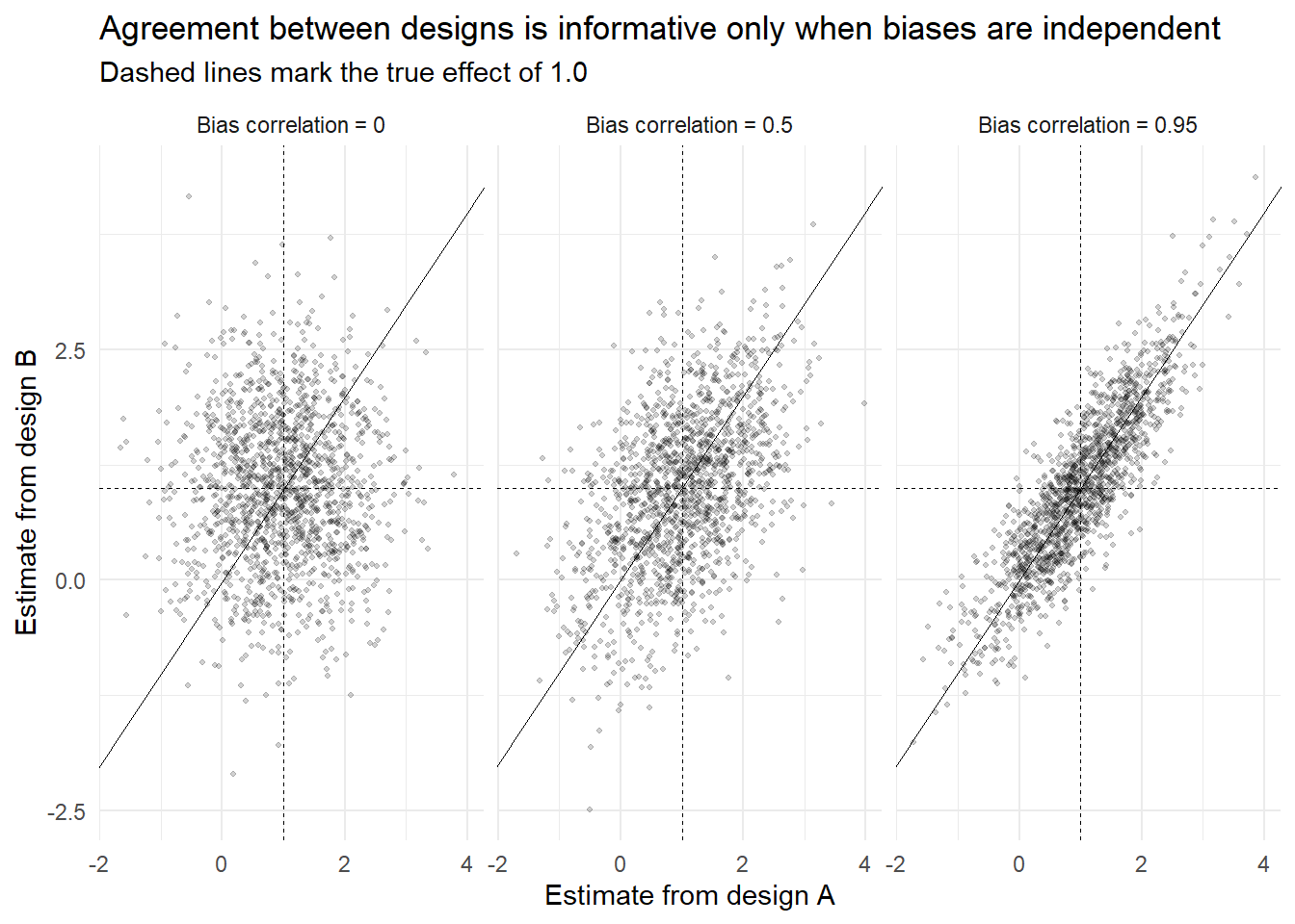
We can quantify the intuition: conditional on the two estimates agreeing closely, how often are they both close to the truth?
Code
diagnostic_value <- function(rho, tol_agree = 0.25, tol_truth = 0.35) {
  d <- simulate_pair(n = 40000, rho = rho)
  agree <- abs(d$est_A - d$est_B) < tol_agree
  both_right <- abs(d$est_A - 1) < tol_truth & abs(d$est_B - 1) < tol_truth
  p_given <- mean(both_right[agree])
  p_uncond <- mean(both_right)
  c(rho = rho,
    P_agree = mean(agree),
    P_right_given_agree = p_given,
    P_right_unconditional = p_uncond,
    lift = p_given / p_uncond)
}

round(t(sapply(c(0, 0.5, 0.95), diagnostic_value)), 3)
#>       rho P_agree P_right_given_agree P_right_unconditional  lift
#> [1,] 0.00   0.165               0.384                 0.107 3.601
#> [2,] 0.50   0.226               0.312                 0.116 2.689
#> [3,] 0.95   0.435               0.278                 0.181 1.537
The last column is the quantity of interest: how much observing agreement raises the probability that both estimates are near the truth. With independent biases, agreement is rare and carries a large lift—seeing it multiplies the odds that both designs are close to right by a substantial factor. As the biases become correlated, agreement becomes common and the lift shrinks toward one: the two designs are converging on each other rather than on the truth, because they are increasingly the same study run twice. The practical instruction is to ask, before running the second analysis, what would make both of these wrong at once—and if the answer is a short list, redesign rather than proceed.
73.4 Inferential Hazards in Multi-Leg Designs
A paper with three legs and several outcomes per leg has many more chances to find something. Three safeguards are now expected.
Multiple hypotheses. Reporting the effect on GPA, on-time graduation, major choice, credits attempted, and retention invites a false positive somewhere. Family-wise error control—stepdown procedures based on the bootstrap rather than a crude Bonferroni correction—preserves power while controlling the error rate (List, Shaikh, and Xu 2019). The code below shows the difference on a set of correlated outcomes.
Code
set.seed(690)

# Five correlated academic outcomes; only the first two carry a true effect.
n <- 2500
treat  <- rbinom(n, 1, 0.5)
common <- rnorm(n)
true_effects <- c(GPA = 0.10, OnTime = 0.09, Major = 0, Credits = 0, Retention = 0)

Y <- sapply(true_effects, function(te)
  te * treat + 0.7 * common + rnorm(n, 0, 1))

pvals <- apply(Y, 2, function(y) coef(summary(lm(y ~ treat)))["treat", 4])

data.frame(
  outcome    = names(pvals),
  p_raw      = round(pvals, 4),
  p_holm     = round(p.adjust(pvals, "holm"), 4),
  p_bh_fdr   = round(p.adjust(pvals, "BH"), 4),
  truth      = ifelse(true_effects > 0, "real", "null")
)
#>             outcome  p_raw p_holm p_bh_fdr truth
#> GPA             GPA 0.0541 0.2162   0.1352  real
#> OnTime       OnTime 0.0079 0.0397   0.0397  real
#> Major         Major 0.4383 0.8765   0.5478  null
#> Credits     Credits 0.2202 0.6606   0.3670  null
#> Retention Retention 0.8281 0.8765   0.8281  null
The instructive pattern is not that correction is conservative—everyone knows that—but which result it kills. The three null outcomes stay null under every procedure, as they should. Among the two real effects, the stronger survives family-wise control and the marginal one does not, which is exactly the situation where a paper is tempted to report the raw p-value and describe the outcome as “marginally significant.” The defensible move is to declare in advance which outcome is primary, control the error rate across the announced family, and label the rest exploratory.
Forking paths. Every leg involves discretionary choices—which cohorts to drop, how to bin income, which covariates to include. Reporting the full distribution of estimates across defensible specifications, rather than one preferred specification plus a robustness table, is now a recognized standard (Simonsohn, Simmons, and Nelson 2020; Steegen et al. 2016). A specification curve is especially valuable in a spillover paper, because the sample-construction choices (Chapter 70) are numerous and consequential.
Pre-specification. Registering the primary outcome, the control group, and the subgroup splits before analysis converts a suggestive complementary result into a confirmatory one, at the cost of flexibility that observational work often needs (Olken 2015). For retrospective administrative-data studies, the practical compromise is to pre-specify the complementary analysis before running it, and to say in the paper that this was done.
The complementary analysis should be pre-committed, not harvested
The strongest version of the third leg is one chosen because the theory predicts it, announced before it is estimated. The weakest is one selected after searching the outcome space for something significant. Since the reader cannot distinguish these from the text, the burden is on the author to make the prediction explicit before the result: the theory says a shift to cheaper financing should relieve liquidity pressure during school, therefore we test achievement outcomes, and therefore a null on major choice is a placebo rather than a disappointment.
73.5 Validating Models Against Held-Out Evidence
A distinct and more demanding form of complementary analysis is to validate the model itself out of sample. The canonical example estimates a behavioral model on pre-experimental data and then predicts the effect of an experiment the model never saw, comparing prediction to realization (Todd and Wolpin 2006). This is the strongest available evidence that a model’s structure, not just its fit, is right.
Marketing has natural opportunities for this that are under-exploited. A firm that calibrates a normative model of customer plan choice can predict the take-up consequence of a plan change before rolling it out, then compare. A platform that models optimal consumer search can predict the effect of a ranking change on an untouched market. The general recipe is: calibrate on period one, predict period two’s policy change, publish the prediction, then report the comparison (DellaVigna 2018). The relationship between such validation exercises and the broader structural-versus-reduced-form debate is the subject of Nevo and Whinston (2010), Angrist and Pischke (2010), and Rust (2014); the practical resolution most policy papers adopt is the one used here—reduced-form evidence for the causal claim, a small model for the welfare claim, and an independent check that the two are consistent.
73.6 A Design Checklist
Table 73.2 converts the chapter into a planning tool. Fill it in before collecting data, not after.
| Question | What to specify in advance |
|---|---|
| What is the primary claim? | One sentence, with the welfare object named |
| What is the primary evidence? | Design, estimand, identifying assumption |
| What is the complementary evidence? | A different data source or design measuring a different construct |
| Are the failure modes disjoint? | List what would have to fail for each; if the lists overlap, redesign |
| Does the complementary leg need its own identification? | Usually yes; name its control group and why it is valid |
| Is there a placebo outcome? | An outcome the theory says should not move |
| How many hypotheses are tested? | Pre-list them; state the multiplicity correction |
| What is the discretion in sample construction? | Enumerate; plan a specification curve |
| Which claims are confirmatory and which exploratory? | Label each in the text |
| What would change your conclusion? | The break-even value of the pivotal input |
73.7 Key Takeaways
- Evidence is complementary only when the assumptions whose failure would invalidate it are largely disjoint from those of the primary analysis; robustness checks that share the identifying assumption are not complementary.
- A strong policy paper has legs that fail for different reasons: a causal design that cannot speak to welfare, a mechanism study that cannot speak to causality, and a downstream-outcome test that cannot isolate mechanism (Table 73.1).
- Linking a survey to administrative records makes belief accuracy observable and is often the only way to detect ignorance-of-own-options as a distinct departure from the normative benchmark.
- The complementary leg usually needs a new identification strategy, and the best source for its control group is a heterogeneity result from the primary leg—a group the first analysis showed was unaffected.
- Include a placebo outcome the theory says should not move; a null there does more for credibility than another significant coefficient.
- Agreement between two analyses is informative only in proportion to how independent their biases are; ask what would make both wrong at once before running the second.
- Control the family-wise error rate across the outcomes a multi-leg design generates, report the specification distribution rather than one preferred model, and pre-commit the complementary test so it reads as confirmatory rather than harvested.
- Out-of-sample validation—calibrate, predict a change the model never saw, then compare—is the most demanding and most persuasive complementary analysis available.
73.8 Further Reading
The three-leg design discussed throughout is Brown, Grodzicki, and Medina (2026). On out-of-sample validation of behavioral models, Todd and Wolpin (2006) remains the reference case, and DellaVigna (2018) surveys the broader practice of combining structure with experimental or quasi-experimental variation. The structural-versus-design debate that frames these choices is set out in Angrist and Pischke (2010), Nevo and Whinston (2010), and Rust (2014). For the inferential hazards, List, Shaikh, and Xu (2019) on multiple hypothesis testing in experimental work, Simonsohn, Simmons, and Nelson (2020) and Steegen et al. (2016) on specification robustness, and Olken (2015) on pre-analysis plans; the marketing field’s own statement on experimental practice is in Nelson, Simester, and Sudhir (2020). The design and estimation background for the individual legs is in Chapter 43 and Chapter 39, and the reporting conventions that make a multi-leg paper auditable are treated in Chapter 77.
Angrist, Joshua D., and Jörn-Steffen Pischke. 2010. “The Credibility Revolution in Empirical Economics: How Better Research Design Is Taking the Con Out of Econometrics.” Journal of Economic Perspectives 24 (2): 3–30. https://doi.org/10.1257/jep.24.2.3.
Brown, Alexander L., Daniel Grodzicki, and Paolina C. Medina. 2026. “When Consumer Financial Protection Spills over: Student Loan Borrowing Under the CARD Act.” Management Science. https://doi.org/10.1287/mnsc.2024.06339.
DellaVigna, Stefano. 2018. “Structural Behavioral Economics.” In Handbook of Behavioral Economics: Applications and Foundations 1, 613–723. Elsevier. https://doi.org/10.1016/bs.hesbe.2018.07.005.
List, John A., Azeem M. Shaikh, and Yang Xu. 2019. “Multiple Hypothesis Testing in Experimental Economics.” Experimental Economics 22 (4): 773–93. https://doi.org/10.1007/s10683-018-09597-5.
Nelson, Leif D., Duncan Simester, and K. Sudhir. 2020. “Introduction to the Special Issue on Marketing Science and Field Experiments.” Marketing Science 39 (6): 1033–38. https://doi.org/10.1287/mksc.2020.1266.
Nevo, Aviv, and Michael D. Whinston. 2010. “Taking the Dogma Out of Econometrics: Structural Modeling and Credible Inference.” Journal of Economic Perspectives 24 (2): 69–82. https://doi.org/10.1257/jep.24.2.69.
Olken, Benjamin A. 2015. “Promises and Perils of Pre-Analysis Plans.” Journal of Economic Perspectives 29 (3): 61–80. https://doi.org/10.1257/jep.29.3.61.
Rust, John. 2014. “The Limits of Inference with Theory: A Review of Wolpin (2013).” Journal of Economic Literature 52 (3): 820–50. https://doi.org/10.1257/jel.52.3.820.
Simonsohn, Uri, Joseph P. Simmons, and Leif D. Nelson. 2020. “Specification Curve Analysis.” Nature Human Behaviour 4 (11): 1208–14. https://doi.org/10.1038/s41562-020-0912-z.
Steegen, Sara, Francis Tuerlinckx, Andrew Gelman, and Wolf Vanpaemel. 2016. “Increasing Transparency Through a Multiverse Analysis.” Perspectives on Psychological Science 11 (5): 702–12. https://doi.org/10.1177/1745691616658637.
Todd, Petra E., and Kenneth I. Wolpin. 2006. “Assessing the Impact of a School Subsidy Program in Mexico: Using a Social Experiment to Validate a Dynamic Behavioral Model of Child Schooling and Fertility.” American Economic Review 96 (5): 1384–1417. https://doi.org/10.1257/aer.96.5.1384.